Scalable Message-Passing Quantum Graph Neural Networks
in the Weisfeiler–Leman Hierarchy

Graphs provide a natural language for relational data in chemistry, biology, and optimisation. Graph neural networks have driven much of the recent progress in learning from such data through message passing, a single primitive that generalises convolution and attention. Quantum counterparts have been proposed, but with limited connection to message passing and few guarantees on performance or scalability. For a quantum model to be useful, it must offer expressivity guarantees together with demonstrable scalability. We show how a quantum graph neural network can be built to perform message passing, to be permutation equivariant, and to sit at a chosen level of the Weisfeiler–Leman hierarchy, the standard measure of how finely a model can tell graphs apart. As for classical graph networks, training can be carried out first on small graph instances, a pre-training that mitigates the usual training difficulties, and the output is read out at a cost that stays low as the graph grows. We validate the framework in large-scale simulations of up to 56 qubits: on synthetic graphs that ordinary message passing cannot separate, on molecular property prediction, and on the travelling salesman problem.

graph learning

Graph neural networks

A graph neural network operates on relational data, such as molecules in drug discovery, interactions in biology, or the road maps behind route optimisation. Almost all such models are built on a single operation, message passing: each node gathers information from its neighbours and updates its own state, and after a few rounds a node’s state summarises its local neighbourhood. For an insightful introduction to graph neural networks, we recommend the Distill primer, A Gentle Introduction to Graph Neural Networks. Three properties make these models effective, and our quantum construction is built to carry all three.

• Message passing. Each node updates its state from its neighbours, $h_i \leftarrow \sigma\!\big(\sum_{j \in \mathcal{N}(i)} A_{ij}\, h_j\, W\big)$, so after $L$ rounds a node’s state summarises its $L$-hop neighbourhood. The rule is local, which is why it scales to large graphs.
• Permutation equivariance. The nodes carry no intrinsic order, so relabelling them by a permutation $\pi$ relabels the output the same way, $f_{\boldsymbol{\theta}}(\pi \cdot G) = \pi \cdot f_{\boldsymbol{\theta}}(G)$.
• Weisfeiler–Leman expressivity. The power to separate non-isomorphic graphs is graded by the $j$-WL hierarchy: when $j$-WL tells two graphs apart, the model does too, $G \not\sim_{j\text{-WL}} G' \Rightarrow f_{\boldsymbol{\theta}}(G) \neq f_{\boldsymbol{\theta}}(G')$.

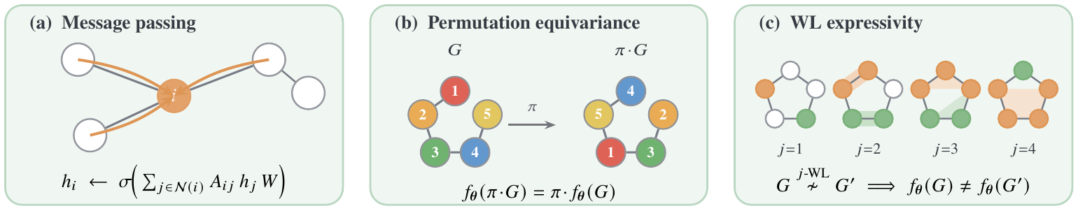
The Weisfeiler–Leman ceiling has an exact form. Message passing separates two graphs only as well as the first level of the hierarchy, the 1-dimensional test (1-WL): if 1-WL assigns two graphs the same final colours, no message-passing network can distinguish them (Xu et al.), and adding layers or widening the hidden dimension does not change this. The limitation has concrete consequences. Two molecules can be genuinely distinct, with different properties, yet present the same colours to 1-WL, so the network returns the same prediction. The same blindness appears in counting: a 1-WL network cannot count cycles, and so cannot distinguish a benzene ring from an open chain of the same atoms.

Expressivity is addressed through the $j$-WL hierarchy, which lifts the test from single nodes to $j$-node subsets, so that a colour describes a group of $j$ nodes rather than one. Larger $j$ resolves edges, triangles, and higher groups, and separates strictly more graphs. In the set-based convention used by the architecture here, the model reaches past the first level at $j \geq 3$.

Quantum graph models also inherit the trainability difficulty common to variational circuits: as the circuit grows, gradients can vanish across parameter space, the barren plateau. It is therefore important to show that a quantum graph model can be both trained and scaled to large graphs. The sections that follow construct a quantum graph network that sits at a chosen level of this hierarchy and remains trainable as it grows.

what the WL test is, and what j-WL adds

The 1-WL test colours nodes by refinement. Every node begins with the same colour. At each step a node is recoloured by combining its own colour with the collection of its neighbours’ colours, keeping repeats but discarding order. Once the colours stabilise, two graphs are declared different only if their colour histograms differ. Message passing is the learned form of this loop, and it inherits the same limitations.

The $j$-WL hierarchy applies the same refinement to $j$-element subsets rather than single nodes. Each subset carries a colour, refined over its one-swap neighbours, the subsets obtained by replacing a single node. A single node at $j{=}1$, an edge at $j{=}2$, a triangle at $j{=}3$: larger $j$ resolves larger structure and separates strictly more graphs. In the set-based convention used here, the model reaches past the first level at $j \geq 3$.

the framework

Quantum graph neural network

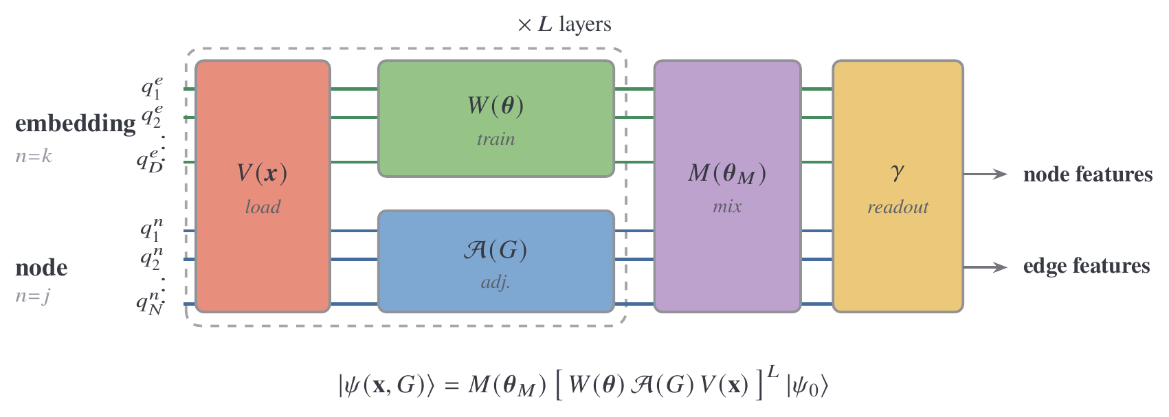
The model divides the qubits into two registers. A node register of $N$ qubits at particle number $j$ holds the graph, spanning a subspace of dimension $\binom{N}{j}$, where the weight $j$ fixes the meaning of a basis state, a single node at $j{=}1$, an edge at $j{=}2$, a triangle at $j{=}3$, and a group of $j$ nodes in general. An embedding register of $D$ qubits at particle number $k$ holds the features, of dimension $\binom{D}{k}$, which sets the model’s capacity and does not grow with the graph. The joint state lies in

$$\dim \mathcal{H} = \binom{N}{j}\binom{D}{k}.$$

One layer, repeated $L$ times, applies four blocks, each with a single role.

• Loader $V(\mathbf{x})$. Writes the graph into the registers, and is re-uploaded at each layer, which makes the input-to-output map nonlinear.
• Adjacency $\mathcal{A}(G)$. Routes amplitude along the edges by Givens rotations between node-qubit pairs in a canonical ordering fixed by the edge weights; a rotation between qubits $a$ and $b$ couples the $j$-subsets that differ by exchanging $a$ for $b$, which is exactly one round of set-based $j$-WL refinement.
• Evolution $W(\boldsymbol{\theta})$. Updates the features on the embedding register only, a compound rotation built from $O = (I-S)(I+S)^{-1} \in SO(D)$, shared across the node components and so independent of the node labels.
• Mixer $M(\boldsymbol{\theta}_M)$. Couples the two registers before the readout.
• Readout $\gamma$. The embedding-register one-body reduced density matrix $\gamma_{pq} = \langle\psi|a_p^\dagger a_q|\psi\rangle$, a $D \times D$ matrix per node, mapped to node and edge features.

The state the circuit prepares is

$$|\psi(\mathbf{x}, G)\rangle = M(\boldsymbol{\theta}_M)\,\big[\, W(\boldsymbol{\theta})\, \mathcal{A}(G)\, V(\mathbf{x}) \,\big]^{L}\, |\psi_0\rangle .$$

Each circuit layer performs one round of set-based $j$-WL refinement, and for $j{\geq}3$ the model separates graphs that 1-WL, and hence every message-passing network, cannot.

Message passing is carried out on the quantum state rather than by a classical post-processing step. In most prior quantum constructions the circuit topology mirrors the graph and the aggregation that defines a graph network is left to a classical readout; the constructions that do aggregate coherently obtain their distinguishing power from random node labels rather than from the aggregation itself. Here the adjacency routes each node’s amplitude along the edges and the evolution updates the per-node features within the circuit, and the classical head only maps the final 1-RDM to node and edge features.

Two properties follow from this structure. Because $\mathcal{A}$ and $M$ order their gates by the graph rather than the labels, and the evolution acts identically on every node’s embedding, relabelling the nodes reorders the same gates without changing their combined action. This construction is therefore exactly permutation equivariant, with no parameters tied. Because every gate preserves particle number, the dynamics remain in the structured subspace above rather than spreading across the full $2^{N+D}$ space, which, on the instances we tested, prevents the gradients from vanishing.

Where the state lives

Each qubit may be read as a slot that is empty ($\ket{0}$) or filled ($\ket{1}$). “Hamming weight $j$” means exactly $j$ slots are filled, and a Givens rotation moves a filled slot to an empty one without changing the count. While a gate acts inside a single register, that register remains on its shell, the conservation a physicist calls fixed particle number.

The mixing layer $M$ couples the registers and conserves only the total weight $j+k$, so the state enters the larger joint subspace of $N+D$ qubits at weight $j+k$, of dimension $\binom{N+D}{j+k}$, still polynomial in $N$ at fixed $(D,k,j)$ and far below $2^{N+D}$, which does not make its classical simulation cheap. The trainability argument rests on the embedding register’s small subspace, whose Lie algebra is polynomial rather than exponential. This is a heuristic supported by numerics, not a confinement theorem. Across the sizes we tested, the measured per-parameter gradient variance remains roughly flat as the joint-subspace dimension grows, rather than decaying as $1/\dim$ as a random initialisation does.

interactive

Subspace

Each gate of the circuit is block-diagonal in the Hamming-weight basis: the full 2ⁿ × 2ⁿ unitary decomposes into one block per particle number, block w having size C(n,w). The coloured block is the subspace in which the model operates. Adjusting N, j, D, k updates the active subspace. Amplitude never leaves the coloured block, so the dynamics stay within this structured subspace. On the instances we test, this keeps the gradients from vanishing as the model grows. The subspace is a small fraction of the full 2ⁿ space, but a small subspace does not make a large instance cheap to simulate classically; that cost grows steeply with size.

Node qubits N

6

Node weight j

3

Embed qubits D

6

Embed weight k

3

node register · W on N qubits

embedding register · W on D qubits

Hamming weight preserved every gate is block-diagonal

S_N-equivariant canonical edge ordering

what we test on

Results

We evaluate the framework on three datasets, each over several random seeds. The travelling salesman problem and QM9 carry the main evaluation, and the Cai–Fürer–Immerman graphs test the $j$-WL ascent directly. The largest run is the travelling salesman problem with 50 cities, which uses 56 qubits, 50 node qubits and 6 embedding qubits.

experiment

Travelling salesman

The Euclidean travelling salesman problem provides an end-to-end test of the framework. The task is to find the shortest closed tour through $N$ cities in the plane, which is NP-hard. The relevant structure is captured at $j{=}1$, so we run the model end to end as a $j{=}1$ instantiation: load the cities, predict which edges belong to the optimal tour, and decode the predictions into a route by beam search of width $100$.

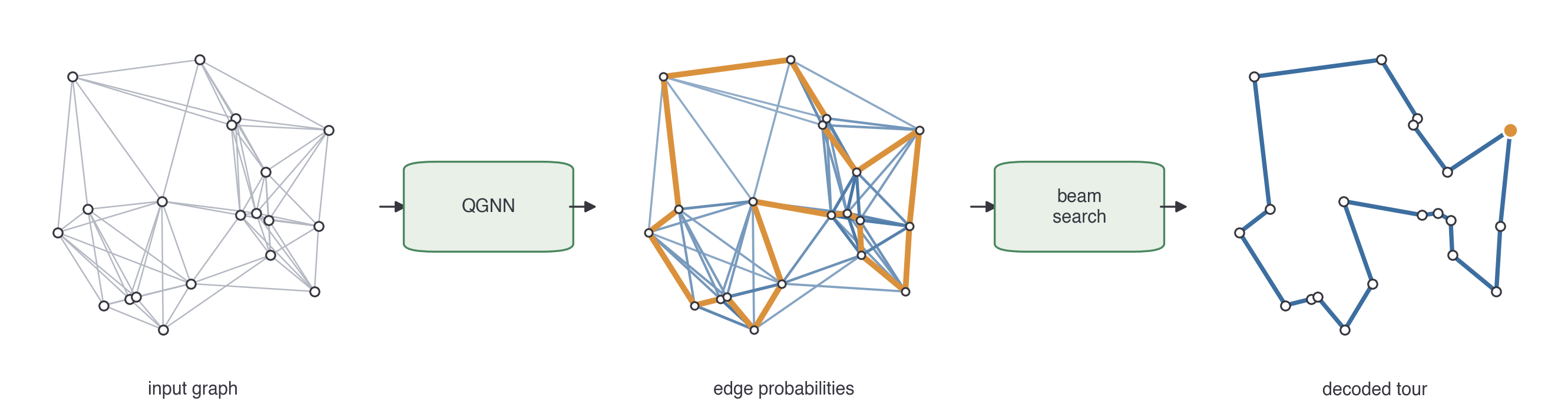
Tour quality is measured by the ratio of the produced tour length to the optimal, where $1.0$ is optimal. The mean ratio is $1.008$, $1.034$, and $1.078$ at $N{=}5, 10, 20$, and rises to $1.128$ and $1.201$ at $N{=}30$ and $N{=}50$, so the quality declines steadily as the graph grows at the fixed embedding. The largest instance, $N{=}50$, is a 56-qubit simulation.

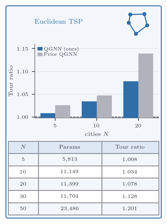
On the three sizes where a quantum baseline can also be simulated, these ratios lie at or below the reinforcement-learning equivariant circuit of Skolik et al., which reaches $1.026$, $1.047$, $1.139$ at $N{=}5, 10, 20$. We run beyond $N{=}20$, where simulating their $N$-qubit state becomes infeasible. The two pipelines optimise different objectives, so this is a comparison of quality rather than a controlled head-to-head.

At matched parameter counts (about $5{,}800$, with the same training set), a classical graph convolutional network achieves a lower edge-prediction loss, test BCE $0.0798$ against $0.224$, roughly $2.8\times$ lower. The $j{=}1$ instantiation is therefore a demonstration that the framework runs end to end and exercises equivariance, trainability, and redeployment, rather than a claim of improved performance over classical networks; this comparison is taken up in the Discussion.

experiment

Molecular property prediction (QM9)

QM9 is a standard chemistry benchmark of 130,831 small organic molecules, each with up to nine heavy atoms and a set of properties computed by density-functional theory. We predict the HOMO–LUMO gap, the energy difference between a molecule’s highest occupied and lowest unoccupied orbitals, which governs much of its reactivity and is a common target for learned property prediction.

Here we ask whether raising the node-register particle number $j$, which raises the model’s $j$-WL level, lowers the error on a real task. Between runs we change only $j$; the embedding, the circuit depth, the readout head, and the optimiser are held fixed.

The test error decreases as $j$ increases: $0.398$ eV at $j{=}1$, $0.308$ eV at $j{=}2$, and $0.235$ eV at $j{=}3$. The $j{=}1$ value is a validation estimate and the other two are test errors. The parameter count changes little across the sweep, from $2{,}591$ to $2{,}655$, so the improvement follows from the added node-register resolution rather than from a larger model.

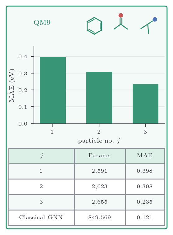
A classical message-passing network reaches a lower error of $0.121$ eV on the same task, but with about $320\times$ more parameters ($849{,}569$ against roughly $2{,}600$). The relevant observation is that the same particle number that raises the Weisfeiler–Leman level on synthetic graphs also reduces the chemical-property error on a real dataset, at near-constant parameter count.

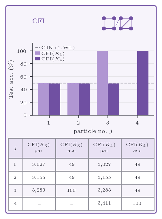
experiment

Distinguishing graphs (CFI)

The Cai–Fürer–Immerman graphs are a direct test of the $j$-WL ascent: pairs of non-isomorphic graphs built so that 1-WL, and every message-passing network with it, cannot tell them apart, so separating a pair requires going beyond 1-WL. We use two families, CFI($K_3$) on $N{=}6$ vertices, separable at $j{=}3$, and CFI($K_4$) on $N{=}8$ vertices, separable at $j{=}4$.

We train the model end to end as a binary classifier on random relabellings of each graph, so success requires a permutation-invariant rule rather than memorised vertex labels. On both families the test accuracy jumps from chance to $100\%$ exactly at the predicted particle number, $j{=}3$ for CFI($K_3$) and $j{=}4$ for CFI($K_4$), and stays at chance below it. A 1-WL graph isomorphism network (GIN) stays at chance on both families, while a 3-WL network (PPGN) separates both, which places the model’s distinguishing power at the level the ascent predicts.

symmetry

Permutation equivariance

The nodes of a graph carry no intrinsic order, and relabelling them yields the same graph. The model must therefore commute with relabelling: permuting the input nodes permutes the output node and edge features in the same way. Building this symmetry into the architecture, rather than learning it from data, excludes functions that disagree under relabelling, which lowers sample complexity and improves generalisation from limited data.

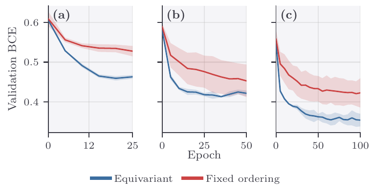
The standard route to permutation symmetry in quantum graph models ties parameters across the symmetric group, for example a fixed number of angles per layer independent of graph size, which contracts the function class more than the symmetry requires and costs expressivity within the equivariant subspace. The architecture here takes a different route, obtaining exact equivariance from the two-register structure with no parameters tied. The adjacency block $\mathcal{A}(G)$ and the mixer $M$ order their gates by a canonical ordering fixed by the graph’s edge weights rather than by the node labels, and the trainable evolution $W$ acts identically on every node’s embedding register, so a relabelling reorders the same gates without changing their combined action, at every parameter value.

We measure the effect on TSP-5 edge prediction. The model scores each edge for membership in the optimal tour, graded by validation loss (lower is better). The equivariant model is compared against a matched-parameter variant that replaces the canonical edge ordering with a fixed-lexicographic one and is otherwise identical. The equivariant model attains a lower validation loss at every training-set size, by $14\%$, $6\%$, and $16\%$ at $n{=}500$, $1000$, and $2000$ (three seeds each); at $n{=}2000$ it reaches $0.354$ against $0.423$. The direction is that expected from a smaller hypothesis class.

scaling

Trainability and readout

Two properties determine whether the framework scales: training must retain a usable gradient as the model grows, and the trained model must admit a cheap readout. Both rest on the same particle-number-preserving Givens gates, and we establish them numerically.

Trainability. A subspace-preserving circuit is expected to avoid the barren plateau, and the measurements confirm this. We measure the per-parameter gradient variance at random initialisation across a range of graph and embedding sizes. At fixed $(D,k)$ the variance is flat in $N$, and across the three operating points $(D,k)\in\{(6,3),(8,4),(10,5)\}$ it remains well above the exponential decay characteristic of a barren plateau, following an inverse-polynomial trend out to $N{+}D=56$ qubits.

Transferred initialisation improves the signal further. Because the trainable weights act on the embedding register, whose size does not grow with the graph, parameters fitted on a small instance can initialise a larger one. Transferring from a single TSP-5-trained model keeps the gradient one to two orders of magnitude above a random start across sizes, which supports a train-small, deploy-large procedure. Chaining the transfer step by step from $N{-}1$ to $N$ performs less well, and is shown for comparison.

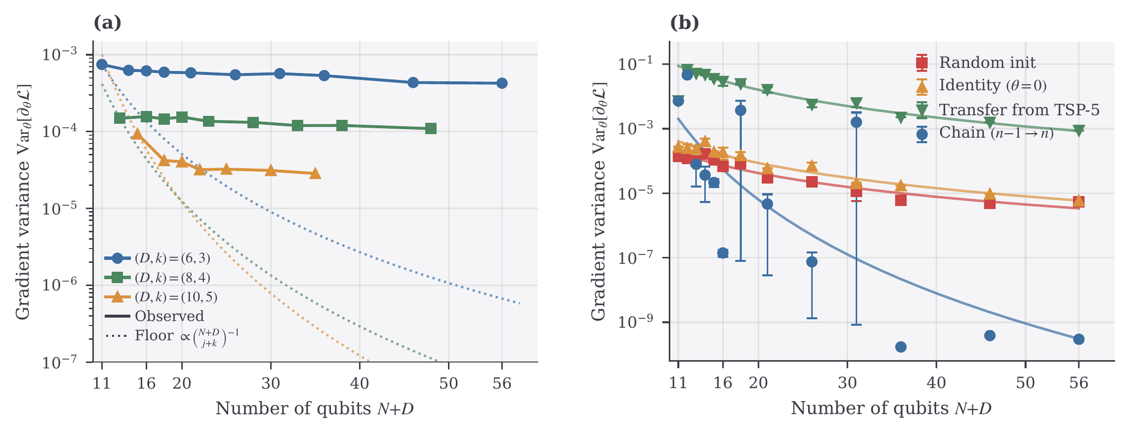
Reaching these sizes in classical simulation is itself demanding. The subspace constraint gives only a polynomial overhead, yet the cost grows steeply with the graph. On our cluster a single configuration takes roughly five minutes at $N{=}20$ (26 qubits), about a day at $N{=}30$ (36 qubits), and weeks at $N{=}50$ (56 qubits). We pushed the simulations to the largest sizes the cluster allowed, in order to follow the trend; a structured subspace does not make a large instance cheap to simulate.

graph size	qubits (N+D)	classical simulation
N = 20	26	~5 minutes
N = 30	36	~1 day
N = 50	56	~weeks

Readout. Deployment requires a feature that is inexpensive to measure. That feature is the embedding-register one-particle reduced density matrix $\gamma_{pq}=\langle\psi|a_p^\dagger a_q|\psi\rangle$, a $D \times D$ matrix per node, with trace $k$ and eigenvalues in $[0,1]$. It is read in two steps: projecting the node register onto a single node, then measuring the embedding register of the conditional state. The matrix is estimable to accuracy $\epsilon$ in $O(D^3/\epsilon^2)$ shots, either by a deterministic Hartree–Fock readout or by a matchgate shadow. The cost is set by the $D$-qubit feature register, so it is polynomial in $D$ rather than the $\binom{D}{k}^2$ of full tomography, and it does not grow with the number of nodes. The choice of readout shows up on the task: a computational-basis $Z{+}ZZ$ readout recovers only the diagonal of $\gamma$ and stalls at tour ratio $1.043$ on the travelling-salesman task, while the Hartree–Fock and matchgate-shadow readouts recover the full matrix and reach $1.006$ at the same shot budget. This readout is intended for hardware deployment; it is defined and benchmarked here, and not run on hardware in this work.

code

Data loader

The loader writes the graph into the circuit. It is a controlled-Givens particle-number encoder: each city’s coordinate embedding is placed into a fixed-particle-number subspace and retained there, and it is re-uploaded at every layer, so that later layers act on a richer function of the coordinates. We provide two back-ends for the same map: a PennyLane circuit defined gate by gate, and a vectorised PyTorch implementation that performs the same algebra without constructing a state vector.

PennyLane loader

Each register block encodes data into the weight-$k$ subspace with $k = D/2$. At $(D,k)=(6,3)$ that subspace has $\binom{6}{3}=20$ basis states, so the loader needs exactly $19$ Givens rotations to traverse them. The traversal follows an Ehrlich Gray sequence: consecutive basis strings differ in exactly two bit positions, so a single qml.SingleExcitation rotates between them.

def hierarchical_loader_ops_batched(bottom_weights, top_data, n, D, is_initial_load=True):
    k_top = D // 2
    # --- bottom register: unary city index in the HW=1 subspace ---
    bottom_strings, bottom_path = get_ehrlich_paths(n, 1)
    bottom_angles = generate_angles(preprocess_data(bottom_weights, n))
    if is_initial_load:                       # HW-init X gate ONLY on the first layer
        qml.X(n - 1)
    for idx, (tgt, _) in enumerate(bottom_path):
        qml.SingleExcitation(bottom_angles[idx], wires=[tgt[0], tgt[1]])

    # --- top register: embedding in the HW=k subspace, controlled on the city ---
    _, top_path = get_ehrlich_paths(D, k_top)
    for i, bottom_string in enumerate(bottom_strings):
        ctrl = bottom_string.find('1')        # which city this branch encodes
        angles = generate_angles(preprocess_data(top_data[i], comb(D, k_top)))
        if is_initial_load:                   # set HW=k, once
            for j in range(k_top):
                qml.ctrl(qml.X(n + D - 1 - j), control=ctrl)
        for idx, (tgt, c) in enumerate(top_path):
            qml.ctrl(qml.SingleExcitation(angles[idx], wires=[n+tgt[0], n+tgt[1]]),
                     [ctrl, *[n+x for x in c]])

Two features of this construction are essential. First, SingleExcitation is a particle-number-conserving rotation: $\ket{01}$ and $\ket{10}$ mix, $\ket{00}$ and $\ket{11}$ are fixed, so the Hamming weight is unchanged. Second, is_initial_load gates the X gates, which run on the first layer to prepare the subspace and are skipped on every re-upload, since the state is already in the subspace.

PyTorch loader

HierarchicalLoader precomputes, for each Ehrlich gate, the index pair $(i,j)$ it acts on, then applies every rotation as gather / rotate / scatter on a $[B, N, d]$ tensor. The $N$ cities and the $d$ embedding amplitudes are separate axes, so no $2^{N+D}$ vector is allocated.

for gate_idx in range(num_gates):
    idx_i, idx_j = basis.gate_indices_i[gate_idx], basis.gate_indices_j[gate_idx]
    theta = angles[:, :, gate_idx]                      # [B, N]
    c, s = torch.cos(theta/2).unsqueeze(-1), torch.sin(theta/2).unsqueeze(-1)
    vi, vj = X[:, :, idx_i], X[:, :, idx_j]             # gather the two amplitudes
    X = X.scatter(2, idx_i_exp, c*vi - s*vj)            # rotate, write back; no .clone()
    X = X.scatter(2, idx_j_exp, s*vi + c*vj)

A Givens rotation that mixes only equal-weight basis states cannot leak amplitude out of the subspace, so a norm check on the reconstructed state confirms the invariant: at $N=3$, $(D,k)=(6,3)$, an initial load followed by a re-upload keeps the total Hamming weight fixed, with a double-precision residual at machine epsilon.

code

Adjacency, evolution, and readout

Three further blocks turn the loaded state into a graph-aware prediction. Each reuses the loader’s pattern, gathering a few amplitudes by precomputed index, rotating them in a plane, and scattering them back. Each is described briefly, with the code that implements it.

Equivariant adjacency, $\mathcal{A}(G)$. The graph enters as Givens rotations on node-qubit pairs. A rotation between qubits $a$ and $b$ couples the node subsets that differ by exchanging $a$ for $b$, which is one round of $j$-WL refinement on the state. The ordering of these rotations is essential, since rotations in different planes do not commute and the order changes the result. If the layer ordered edges lexicographically by qubit index, relabelling the nodes would reorder the gates and change the circuit’s output, breaking equivariance. The layer instead sorts edges by a key derived from the edge weights (descending in weight, lexicographic only to break ties). Under a relabelling of the nodes the same gates are applied in the same order, so the output is the relabelled output of the original.

# EquivariantAdjacencyLayer.forward (condensed)
sorted_i, sorted_j = self.orient_and_sort_edges(coords)  # canonical edge order
angles = self.compute_angles(coords, sorted_i, sorted_j) # per-edge MLP, tanh*pi/2
for e in range(self.num_edges):
    i, j, th = sorted_i[:, e], sorted_j[:, e], angles[:, e]
    c, s = torch.cos(th/2)[:, None], torch.sin(th/2)[:, None]
    Xi, Xj = X[arange, i], X[arange, j]                  # gather two node rows
    X = X.scatter(1, i_exp, (c*Xi - s*Xj)[:, None])      # rotate, functional scatter
    X = X.scatter(1, j_exp, (s*Xi + c*Xj)[:, None])

Trainable evolution, $W$. This block updates the features and acts on the embedding register only, so it is independent of the node labels. Each block is a single $D \times D$ rotation $O \in SO(D)$, built from a skew-symmetric matrix by the Cayley map $O=(I-S)(I+S)^{-1}$. On the weight-$k$ subspace it acts as a $\binom{D}{k} \times \binom{D}{k}$ orthogonal transform built from the $k \times k$ minors of $O$, a compound representation. Thus $D(D-1)/2$ parameters drive the full $\binom{D}{k} \times \binom{D}{k}$ map: at $(D,k)=(6,3)$, $15$ parameters drive a $20 \times 20$ transform.

O = cayley(build_skew(self.skew_params))     # SO(D), D(D-1)/2 params
C = compound(O, k)                           # C(D,k) x C(D,k), minors of O
return X @ C.T                               # apply to weight-k state

This restriction is deliberate. At $(D,k)=(6,3)$ the block generates $\mathfrak{so}(6)$, of dimension $15$, whereas an unconstrained layer on the same $20$-dimensional subspace would reach $\mathfrak{so}(20)$, of dimension $190$. We retain the smaller algebra: it is less expressive, but its gradients are substantially larger, which preserves trainability as the model grows.

Readout, the 1-RDM. The feature read out for hardware is the one-body reduced density matrix $\gamma_{pq}=\langle\psi|a_p^\dagger a_q|\psi\rangle$, a $D \times D$ matrix per node, with trace $k$ and eigenvalues in $[0,1]$. It can be estimated from a Hartree–Fock state or a matchgate shadow in $O(D^3/\epsilon^2)$ shots, polynomial in $D$ rather than the $\binom{D}{k}^2$ of full tomography. It is defined and benchmarked here, and not run on hardware in this work.

# embedding-register 1-RDM per node, gamma[p,q] = <psi| a_p^dag a_q |psi>
# deterministic Hartree-Fock / matchgate-shadow readout (see matchgate_shadows.py)
gamma = CovarianceComputer(D, k).compute(psi)  # D x D, trace = k, eigvals in [0,1]
node_feats = gamma.reshape(B, N, D * D)        # per-node feature for the readout MLP

discussion

Discussion

The framework adapts the structure and theoretical guarantees of graph neural networks from the classical literature to quantum circuits. It represents and processes graphs in a similar way, and recovers the properties that the classical literature identifies as the ones a graph neural network should have: message passing, in which each node gathers information from its neighbours and updates its state; permutation equivariance, in which relabelling the nodes relabels the output the same way; and Weisfeiler–Leman expressivity, the standard measure of how finely a model distinguishes graphs.

We give several constructions, based on subspace-preserving gates, that prove these properties hold for a quantum graph network. The circuit performs message passing within the quantum state: the adjacency layer routes node amplitudes along the edges, the trainable evolution updates the per-node features, and re-uploading the graph at each layer makes the map nonlinear, with one circuit iteration corresponding to one round of set-based refinement. The construction is exactly permutation equivariant at every value of the parameters, without tying or sharing weights, which is how earlier equivariant models impose the symmetry. To our knowledge it is the first quantum graph model proven to exceed the 1-WL ceiling, and the same approach can be carried to other subspace-preserving architectures.

We validated these properties numerically on three datasets, two of them with real-world applications, with good results on large models of up to 56 qubits. On the Cai–Fürer–Immerman graphs, constructed so that no 1-WL network can separate them, the model distinguished the pairs at exactly the level the ascent predicts. On QM9, where the task is to predict the HOMO–LUMO gap, the error decreased as we raised the particle number at a fixed parameter budget. On the Euclidean travelling salesman problem, the model produced near-optimal tours up to the largest instances we were able to simulate. Together with the theoretical motivation, these results show how the framework can provide quantum methods that scale beyond small proofs of concept.

Finally, the approach is motivated by its scalability. Across every configuration we trained, the per-parameter gradient did not vanish as the subspace dimension grew. The barren-plateau results in the literature characterise broad families of variational circuits, typically generic or randomly initialised ansätze; our model is not of that kind, since its graph information enters through a fixed initialisation and its trainable dynamics stay within a small structured register. The trainability we observe therefore sits alongside those results rather than against them: the general theory bounds what happens across a class, but it does not settle what a specific, structured instantiation does in practice, and the favourable behaviour we find is of that practical kind. The graph-style pre-training used here, where parameters fitted on small instances seed larger ones, is one way to preserve this behaviour as the graph grows, and it invites a theoretical treatment aimed at structured, pre-trained circuits rather than generic ones.

references

References

• Gilmer et al. Neural Message Passing for Quantum Chemistry (2017).
• Xu et al. How Powerful are Graph Neural Networks? (2019).
• Morris et al. Weisfeiler and Leman Go Neural (2019).
• Cai, Fürer, Immerman. An optimal lower bound on the number of variables for graph identification (1992).
• McClean et al. Barren plateaus in quantum neural network training landscapes (2018).
• Cherrat et al. Quantum Vision Transformers (2024).
• Skolik et al. Equivariant quantum circuits for learning on weighted graphs (2023).
• Ramakrishnan et al. Quantum chemistry structures and properties of 134 kilo molecules (2014).

citation

Citation

@article{raj2026qgnn,
  title   = {Scalable Message-Passing Quantum Graph Neural Networks in the
             Weisfeiler--Leman Hierarchy},
  author  = {Raj, Snehal and Coyle, Brian and Monbroussou, L{\'e}o and
             Ferreira-Martins, Andr{\'e} J. and Farias, Renato M. S. and
             Kashefi, Elham},
  year          = {2026},
  eprint        = {2606.26873},
  archivePrefix = {arXiv},
  primaryClass  = {quant-ph}
}

data and code availability

The travelling-salesman instances are taken from the equivariant quantum circuit benchmark of Skolik et al. QM9 is loaded from the standard PyTorch Geometric distribution. The CFI families are generated programmatically from the Cai–Fürer–Immerman construction, and the BREC pairs are taken from the BREC benchmark. The framework (a vectorised PyTorch back-end for $j{=}1$ and a PennyLane reference for $j{\geq}2$) and the readout protocols are released under the MIT licence at github.com/SnehalRaj/mp-qgnns, with scripts to reproduce each reported result.